Climate modelling

Climate and its volatility

Climate is not constant in time or space. The climate of a planet goes through natural changes in the course of its history, just like Earth in the past millions of years. Paleoclimatology deals with the study of the past climate of the Earth, where glacial and interglacial periods changed each other. Ice samples from the Antarctic show that during the last 500000 years Earth witnessed four full glacial periods. Most recent research indicated that in the course of the last glacial period, extreme temperatures in both directions have been changing each other very rapidly, especially on the Northern hemisphere. However, the last 10000 (apart from some significant but local changes) can be considered much more stable and balanced. Northern hemisphere has been characterised in the last 1000 years by an irregular but constant cooling which was followed by a massive warming in the 20th century. In the 11th and 13th centuries, average temperatures were relatively high, while relatively low temperatures could have been observed in the 16th and 19th centuries (small ice age). Changes in temperature at both hemispheres have just one thing in common: the excessive warming in the 20th century could have been observed on both hemispheres.

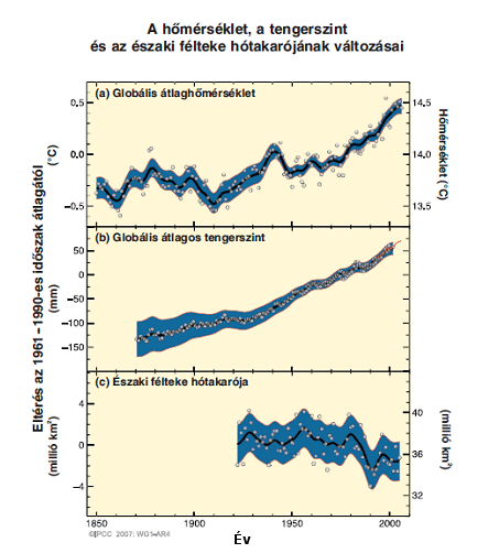
Observed changes in global average temperatures (a), rise in global mean sea level (b) based on tide-ebb meters (blue) and satellite measurements (red, starting from 1978), and changes in the March snow cover of the Northern hemisphere (c). Changes are relative to the respective averages calculated for the 1961-1990 period. Circles indicate annual averages while smoothed curves depict the average values of decades. Areas with grey shades indicate estimated uncertainties. (Source: IPCC, 2007)

Based on the data of instrumental measurements becoming more systematic and frequent since the middle of the 19th century, warming of the Earth’s atmosphere can be clearly indicated. The pace of warming however became frightening for today. Recognizing the serious problems of climate change, the IPCC (Intergovernmental Panel on Climate Change, established in 1988) set the objective to summarize and publish the results of research on climate.

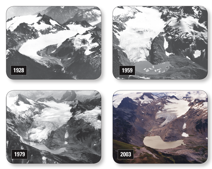
The South Cascade glacier (Washington, USA) in the last century, and its significant withdrawal until the beginning of the 21st century. ( Source: USGS Fact Sheet 2009-3046)

The four IPCC reports published up to now (1990, 1996, 2001 and 2007) provide scientifically based information on the expected impacts of climate change, and provide help for the adaptation to the expected challenges. On average, global mean temperature has been risen by 0.7°C during the 20th century. However, in the last century, this growth was not monotonous, shorter or longer cooler and warmer periods followed each other on the back of general warming. The cooler period at the beginning of the century was followed by a warming of around 0.5°C until the end of the 1940’s, but then again, a cooler period could have been observed. From the 1980’s on, the pace and extent of warming have been above average. Almost in all cases, the current year is the warmest year since the beginning of instrumental measurements. (This is supported by the fact that the warmest registered decade was the last one, 2001-2010.) The fact of increasing surface temperatures was supported also by the most thorough ever analysis made on the climate of the past 200 years by the group led by Richard Muller, a physicist at Berkeley University, California. The study, published in October, 2011, was made by using 1.6 billion data from 39028 weather stations. Their results indicated that the temperature of land areas increased by approximately 1°C since the middle of the 1950’s.

According to the model estimates in the IPCC reports, the frequency and intensity of extreme weather events can also increase in the near future, which urge the analyses on regional scales and the study of adaptation options. The third IPCC report published in 2001 called public attention that based on long-term model results and theoretical assumptions, numerous regions of the Earth are going to become vulnerable due to global warming. In this report, the endangered regions include the countries of Central East Europe and the region of the Mediterranean Sea. Therefore, it is imperative to make regional climate scenarios for the region of the Carpathian basin. The following part is going to describe what kind of tools we have to describe expected future changes of climate.

Climate modelling

Scientists employ computer models to assist in a wide variety of tasks, including forecasting day to day weather, analyzing local severe weather events, predicting future climates, and even modelling the atmospheres of different planets. Shortly after the invention of the computer however, scientists' goals were more humble, since they rarely had much more than a few bytes of memory to work with and had to spend a significant amount of time repairing hardware.

In the mid-20th century, as the idea arose that computers could perform the myriad calculations to simulate atmospheric motion, scientists attempted to apply the pre-defined laws of physics and fluid dynamics to recreate large scale atmospheric circulation. After several attempts they soon learned that the atmosphere was much more complex than their simple models could handle. They were greatly limited by computer technology and more importantly lacking in important knowledge of how climatic processes interact and how they influence climate. On one of the early forecast models, run on ENIAC (electronic numerical integrator and computer), one of the first computers, the modellers found that a two dimensional simulation with grid points 700km apart with 3 hour time steps could forecast for a 24 hour period in about 24 hours, meaning that the model was just able to keep up with the weather as opposed to creating useful forecasts days in advance. Models were indeed simple compared to today; for example, after several failed attempts to create a basic representation of large scale atmospheric flow, scientists at Princeton University's Geophysical Fluid Dynamics Laboratory (GFDL) created a model that incorporated large eddies, making the simulation much more representative. This experiment was deemed a major success and the model is considered the first true GCM. It showed scientists just how significant transient disturbances and smaller scale processes are in influencing the transportation of energy and momentum throughout the atmosphere.

With this success research groups around the country began to develop their own models, including at UCLA's Lawrence Livermore National Laboratory (LLNL) and the National Center for Atmospheric Research (NCAR), further adding to the resources attempting to accurately forecast weather and model the climate system. With a greater number of scientists working on the problem, more was learned about the climate system and progress accelerated. In addition, the rapid increase in computer technology, from the few bytes of memory the first modellers had to work with, to kilobytes, megabytes, and gigabytes, enabled the creation of much more complex models.

Even with drastic advances in technology and scientific knowledge, climatologists still have to make many compromises in terms of realistically representing the Earth. For example, until recently most models focused only on atmospheric circulation (AGCMs) whereas we now know that the oceans, cryosphere (glaciers, ice sheets, sea ice, snow cover), and land surface play extremely important roles in shaping our climate. Today, most models contain a separate or self-contained oceanic component that actively interacts with the model atmosphere. These are called Atmosphere-Ocean coupled models, or AOGCMs.

While early modellers made significant progress, the models still had problems reliably forecasting climatic trends or oscillations. Because the model resolution was extremely coarse many processes had to be parameterized. Model resolution is analogous to photographic resolution as a measure of how small you can look at details. In computer models resolution is important for small scale disturbances like thunderstorms and cyclones and also for accurate representation of the Earth. For example, in early GCMs the land surface resolution was so coarse that peninsulas and islands such as Florida and the UK did not exist and the Great Lakes were treated as land. While extremely fine resolution may be ideal, a balance must always be struck between model resolution and the computer power available. If a model takes months to run then it's not useful to modellers trying to do experiments. The computer power/resolution balance can be thought of as follows: for every doubling in spatial resolution (horizontal and vertical) there is an eightfold increase in grid points to solve for, and very often to keep the model mathematically stable the time step must be halved as well, meaning you would need 16 times more computer power just to double your model resolution.

The process whereby model resolution forces climatologists to simplify calculations is called parameterization. It is the recognition that, while we realize there is an important process here and we have an idea of its magnitude, we cannot possibly explicitly model it so we must attempt to treat it as realistically as possible. One important example of a parameterized process is convective clouds and thunderstorms. Thunderstorms, while extremely important in the atmosphere for transporting heat and water vapour, are also extremely small on the global-scale. A typical GCM grid box ranges from 100km - 300km and the typical thunderstorm is around 1km. Therefore convection must be treated in a much simpler way. While it seems unlikely and maybe unnecessary for convective clouds to ever be modelled in a GCM, parameterizations have also evolved over time and have become better at calculating the influence convection has in the atmosphere.

In the late 20th century, as models and computers became more complex and powerful, model design began to diverge into several subcategories focusing on different aspects of weather and climate, including Numerical Weather Prediction models (NWP), regional scale models, and mesoscale models. These models all differ from GCMs in that they focus on different aspects of the atmosphere. For instance, NWP models use a much smaller horizontal scale--the North American continent for example--and attempt to forecast small changes in weather over short periods of time (a few hours or days). These differ from GCMs in that they are highly sensitive to initial conditions, where meteorological data fed into the model have a dramatic influence on the output. These models deal with what is called the "initial value" problem in that, given meteorological data, the simulation will diverge from reality over time. Climate models are less dependent upon initial conditions and instead must deal with the "boundary value" problem. This occurs where, once the general circulation of the atmosphere has been established, it is difficult to create realistic climatic disturbances such as interannual oscillations (ENSO, PDO, NAO) or climatic trends caused by external forces.

Slowly but surely models have been developed, refined, and tested against real-world situations, to the point that in the 1990s many scientists say the modern GCM was established. While some model weaknesses persist in that they may have biases with parameters, such as too much rain in a region or too warm in another, atmospheric scientists have been able to include more and more climatic processes and better simulate the climate as we learn more about our environment and the importance of the terms in the equations.

Climate models

Depending on the various examinations and the objectives to be achieved, different classes of climate models have been established in the past decades. Models in one of these groups are only able to report the thermal characteristics of the climate system, these are called thermodynamic models. Models in a second class, called dynamic models are also able to simulate both thermal processes and flows.

It is often convenient to regard climate models as belonging to one of four main categories:

• energy balance models (EBMs)
• one dimensional radiative-convective models (RCMs);
• two-dimensional statistical-dynamical models (SDMs)
• three-dimensional general circulation models (GCMs).

These models are listed in increasing order of complexity and computational intensity.

It is useful to remember that one need not always necessary to use the most complex model.

Construction of a Modern Climate Model

As climate models evolved through the 1990s, scientists began to shift focus from reproducing general circulation to experimenting with the feedbacks of climatic processes due to increasing greenhouse gases, changing ocean currents and the way the model responds to forced perturbations such as ENSO. As the next generation of models come out improvements in the models make them more reliable for global predictions and more capable of regional analyses. Here is a simplified description of the anatomy of the latest version of the Community Climate System Model: CCSM3

At their core, all GCMs employ a specific set of primitive dynamic equations, which allow the atmosphere to move in three dimensions, warm up and cool down, and transport moisture, etc. These equations are solved over and over again at specified locations in the model's three-dimensional space. There are two main methods for establishing the horizontal domain of a model. The simplest is to establish a grid along lines of latitude and longitude. For example, the CCSM3 can be run on a 2o x 2.5o grid. Another method is to treat atmospheric motion as waves using Fast Fourier Transforms (FFTs) to make the spectral conversion. The resolution then is represented as the number of waves that can be represented around the earth. The CCSM3 uses wave numbers of T31, T42, and T85; where T represents the triangular truncation of the Fourier transform. This resolution can be approximated to longitude/latitude with a resolution of T31 and T85 is 3.75o and 1.41o respectively.

The vertical domain in the CCSM3 is represented by 26 levels, but is complicated by the fact that the atmosphere is compressible and gets exponentially less dense as you move up in altitude. Therefore, the model levels are irregularly spaced so as to have the most levels in the troposphere where most of the weather and interaction between climatic processes occurs. In addition, topography on the Earth's surface creates difficulties with using pressure as the vertical coordinate because in many locations the ground intersects pressure levels. The CCSM3, as most models, uses a variation of the terrain following coordinate called sigma ( and is defined as:

σ = p/ps

where p = pressure and ps = pressure at the surface.

After the atmospheric core of the model has been constructed modellers must try to incorporate all of the other climatic processes and feedback mechanisms that influence climate so as to have an accurate, dynamic representation of the climate system. While the models of the past focused on the atmosphere and sometimes included the oceans, today's models contain separate modules for the land surface, oceans, and sea ice and sometimes include atmospheric chemistry and advanced treatment of aerosols.

The land surface component of the CCSM3 uses the same horizontal grid as the atmospheric component and has 10 subsurface layers to account for soil-atmosphere interactions. The land surface can also be classified as a variety of types including ice, water, urban, and vegetation. These distinctions are important for the radiation balance because the albedo of the land surface can change dramatically. For example, the albedo of urban black top is very close to 0, meaning it absorbs almost all radiation whereas the albedo of snow cover or white sand is closer to 1 meaning it reflects most radiation.

The ocean and sea ice modules of the CCSM3 use a slightly different horizontal grid from the atmosphere, although they have similar horizontal resolution. In addition, the ocean component uses either 25 or 40 vertical levels defined by depth, extending down to the ocean's deepest basins.

These components make up the newest version of the CCSM3 GCM and can be run in different configurations, primarily by varying the horizontal and vertical resolutions. It should be noted, however, that running the finest resolution configuration takes more than 1100 hours of computer time to simulate one year of the atmosphere. That is approximately 46 days and experiments looking at trends even 10 years into the future take significant time to complete. That is why, for the longer period experiments, scientists use the more coarse resolution.

GCMs have become integral for helping scientists study the Earth's large-scale circulations, forecasting interannual variability such as ENSO, and evaluating the possibility of climate change in the decades to come. GCMs differ from other models mostly in their spatial and temporal domains and the inclusion of many processes not needed for other models because of the longer time scales involved. Their spatial domain covers the whole globe as opposed to, for example, a numerical weather prediction (NWP) model which may cover only North America. On the temporal scale they attempt to simulate earth's atmosphere from periods of several months to several decades, whereas NWP models can forecast for periods as short as a few hours and up to several days relatively well.

Global climate models (GCMs)

Climate models are a mathematical representation of the climate. In order to be able to do this, the models divide the earth, ocean and atmosphere into a grid. The values of the predicted variables, such as surface pressure, wind, temperature, humidity and rainfall are calculated at each grid point over time, to predict their future values. The time step (the interval between one set of solutions and the next) is a function of the grid size: the finer the resolution the shorter the interval between each computation. For example, a model with a 100 km horizontal resolution and 20 vertical levels, would typically use a time-step of 10–20 minutes. A one-year simulation with this configuration would need to process the data for each of the 2.5 million grid points more than 27 000 times – hence the necessity for supercomputers. In fact it can take several months just to complete a 50 year projection.

Climate models have been developed from weather forecasting models but, due to the large number of calculations involved, climate models currently use bigger grid spacing and longer time steps so that they can be run further ahead in time for a given amount of computer time. Without more powerful computers, simulation of the climate with the same detail as in weather forecasts would take far too long, especially if we want to explore many different scenarios of the future. Nevertheless, there is increasing convergence between weather forecasting and climate models, especially for predictions in the range out to months and seasons.

Parameterization

There are certain physical processes that act at a scale much smaller than the characteristic grid interval (e.g. clouds and turbulence). And if the complete physics of these processes, for example, clouds, were to be computed explicitly at each time step and at every grid-point, the huge amount of data produced would swamp the computer. These processes cannot be eliminated, so simplifying equations are developed to represent the gross effect of the many small-scale processes within a grid cell as accurately as possible. This approach is called parameterization. There is a lot of research going on to devise better and more efficient ways for incorporating these small scale processes into climate models.

Coupled model systems

Weather forecasting models must handle the properties of the atmosphere in three dimensions, and work with current analyses of the ocean surface temperatures and at least some basic land surface processes. These models have come to be known as atmospheric general circulation models (GCMs). In parallel, studies of the oceans can concentrate on three-dimensional properties of the oceans and are generally known as ocean GCMs. When it comes to simulating the general behaviour of the climate system over lengthy periods, however, it is essential to use models that represent, and where necessary conserve, the important properties of the atmosphere, land surface and the oceans in three dimensions. At the interfaces, the atmosphere is coupled to the land and oceans through exchanges of heat, moisture and momentum. These models of the climate system are usually known as coupled GCMs.

Coupling the ocean processes to atmospheric GCMs is a major challenge. The thermal capacity of the oceans is massive compared to the atmosphere and can provide to, or extract from, the atmosphere, massive amounts of latent and thermal heat. Representing their heat storage, and the absorption of greenhouse gases by the oceans, in long-term simulations of climate requires a full three-dimensional ocean model, which simulates even the deep currents. Changes in the intensity and location of deep-water currents can ultimately have profound effects on the atmosphere. In the past, changes in the circulation of the oceans have produced major atmospheric responses.

The models must also be able to handle shorter-term fluctuations such as those associated with ENSO. Recent developments in climate modelling, which take into account not only surface processes at the ocean-atmosphere interface but also those acting at depth, have produced considerable improvement to the quality of climate model results. An oceanic GCM typically requires very high spatial resolution to capture eddy processes associated with the major currents, bottom topography and basin geometry. High-resolution ocean models are therefore at least as costly in computer time as are atmospheric GCMs. Further coupling of other climate system component models, especially the cryosphere and the biosphere, are also necessary to obtain more realistic simulations of climate on decadal and longer timescales.

Improvement in the horizontal resolution of the global climate models used in the four published PCC reports. The initial 500 km resolution improved to approximately 100 km in 2007. (Source: IPCC, 2007)

Regional Climate Models (RCMs)

Simulating climate change at the regional and national levels is essential for policymaking. Only by assessing what the real impact will be on different countries will it be possible to justify difficult social and economic policies to avert a dangerous deterioration in the global climate. Furthermore, understanding processes on the regional scale is a crucial part of global research. Processes acting on local or regional scales, such as mountain ranges blocking air flow or dust clouds interacting with radiation will ultimately have impacts at the global level.

One technique used to overcome the coarse spatial resolution of coupled GCMs is that of nested modelling, depicted in the image above. This involves the linking of models of different scales within a global model to provide increasingly detailed analysis of local conditions while using the general analysis of the global output as a driving force for the higher resolution model. Results for a particular region from a coupled GCM are used as initial and boundary conditions for the RCM, which operates at much higher resolution and often, with more detailed topography and physical parameterizations. This enables the RCM to be used to enhance the detailed regional model climatology and this downscaling can be extended to even finer detail in local models. This procedure is particularly attractive for mountain regions and coastal zones, as their complexity is unresolved by the coarse structure of a coupled GCM grid.

Climate change scenarios

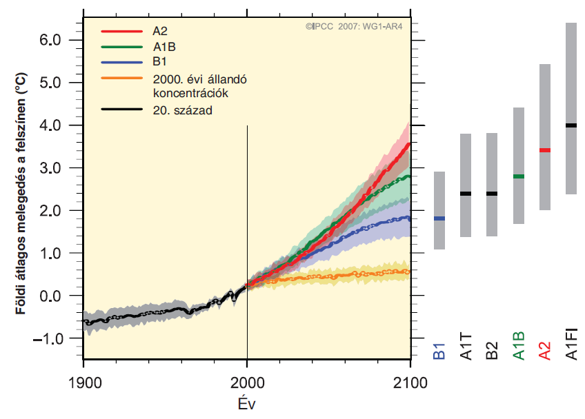
IPCC SRES (Special Report on Emissions Scenarios - SRES) scenarios were constructed to explore future developments in the global environment with special reference to the production of greenhouse gases and aerosol precursor emissions.

The IPCC SRES scenarios contain various driving forces of climate change, including population growth and socio-economic development. These drivers encompass various future scenarios that might influence greenhouse gas (GHG) sources and sinks, such as the energy system and land use change. The evolution of driving forces underlying climate change is highly uncertain. This results in a very wide range of possible emissions paths of greenhouse gases.

The SRES team defined four narrative storylines (see figure below), labelled A1, A2, B1 and B2, describing the relationships between the forces driving greenhouse gas and aerosol emissions and their evolution during the 21st century for large world regions and globally. Each storyline represents different demographic, social, economic, technological, and environmental developments that diverge in increasingly irreversible ways.

The four narrative storylines of SRES

• A1: globalization, emphasis on human wealth Globalized, intensive (market forces).
  The A1 storyline and scenario family describes a future world of very rapid economic growth, global population that peaks in mid-century and declines thereafter, and the rapid introduction of new and more efficient technologies. Major underlying themes are convergence among regions, capacity building, and increased cultural and social interactions, with a substantial reduction in regional differences in per capita income. The A1 scenario family develops into three groups that describe alternative directions of technological change in the energy system. The three A1 groups are distinguished by their technological emphasis: fossil intensive (A1FI), non-fossil energy sources (A1T), or a balance across all sources.
• A2: regionalization, emphasis on human wealth Regional, intensive (clash of civilizations).
  The A2 storyline and scenario family describes a very heterogeneous world. The underlying theme is self-reliance and preservation of local identities. Fertility patterns across regions converge very slowly, which results in continuously increasing global population. Economic development is primarily regionally oriented and per capita economic growth and technological change are more fragmented and slower than in other storylines.
• B1: globalization, emphasis on sustainability and equity Globalized, extensive (sustainable development).
  The B1 storyline and scenario family describes a convergent world with the same global population that peaks in midcentury and declines thereafter, as in the A1 storyline, but with rapid changes in economic structures toward a service and information economy, with reductions in material intensity, and the introduction of clean and resource-efficient technologies. The emphasis is on global solutions to economic, social, and environmental sustainability, including improved equity, but without additional climate initiatives.
• B2: regionalization, emphasis on sustainability and equity Regional, extensive (mixed green bag).
  The B2 storyline and scenario family describes a world in which the emphasis is on local solutions to economic, social, and environmental sustainability. It is a world with continuously increasing global population at a rate lower than A2, intermediate levels of economic development, and less rapid and more diverse technological change than in the B1 and A1 storylines. While the scenario is also oriented toward environmental protection and social equity, it focuses on local and regional levels.

Expected climatic changes in Europe

· Climate change is expected to magnify regional differences in Europe’s natural resources and assets. Negative impacts will include increased risk of inland flash floods and more frequent coastal flooding and increased erosion (due to storminess and sea level rise).

· Mountainous areas will face glacier retreat, reduced snow cover and winter tourism, and extensive species losses (in some areas up to 60% under high emissions scenarios by 2080).

· In southern Europe, climate change is projected to worsen conditions (high temperatures and drought) in a region already vulnerable to climate variability, and to reduce water availability, hydropower potential, summer tourism and, in general, crop productivity.

· Climate change is also projected to increase the health risks due to heat waves and the frequency of wildfires.

References

Adem, J ., 1965: Experiments aiming at monthly and seasonal numerical weather prediction. Monthly Weather Review, 93: 495–503.

Bartholy, J., R. Pongrácz, Gy. Gelybó, 2006a: Regionális éghajlati szcenáriók a PRUDENCE projekt eredményei alapján. In: Napjaink környezeti problémái - globálistól lokálisig: Sérülékenység és alkalmazkodás, CD-ROM. Pannon Egyetem Georgikon Mezőgazdaságtudományi Kar, Keszthely. 6p.

Bartholy, J., R. Pongrácz, Cs. Torma, A. Hunyady, 2006b: A PRECIS regionális klímamodell és adaptálása az ELTE Meteorológiai Tanszékén. In: 31. Meteorológiai Tudományos Napok – Az éghajlat regionális módosulásának objektív becslését megalapozó klímadinamikai kutatások (Weidinger T., szerk.) Országos Meteorológiai Szolgálat, Budapest. 99-114.

Bartholy, J., R. Pongrácz, Cs. Torma, A. Hunyady, 2006c: A regionális klímaváltozás becslése a Kárpát-medence térségére. VAHAVA-zárókonferencia. In: A globális klímaváltozás: hazai hatások és válaszok. KvVM-MTA “VAHAVA” project. (Láng I., Jolánkai M., Csete L., szerk.) CD-ROM. Akaprint, Budapest. 5p.

Bartholy, J., R. Pongrácz, Cs. Torma, I. Pieczka, P. Kardos, A. Hunyady, 2009a: Analysis of regional climate modeling experiments for the Carpathian Basin. Int. J. Global Warming, 1: 238-252.

Bartholy, J., G. Csima, A. Horányi, A. Hunyady, I. Pieczka, R. Pongrácz, Cs. Torma, G. Szépszó, 2009b: Regional climate models for the Carpathian basin: validation and preliminary results for the future. EGU2009-12509. Geophysical Research Abstarct, 11, 12509. CD-ROM. EGU General Assembly 2009.

Beniston, M., D.B. Stephenson, O.B. Christensen, C.A.T. Ferro, C. Frei, S. Goyette, K. Halsnaes, T. Holt, K. Jylhä, B. Koffi, J. Palutikof, R. Schöll, T. Semmler, K. Woth , 2007: Future extreme events in European climate: An exploration of regional climate model projections. Clim. Change, doi:10.1007/s10584-006-9226-z.

Budyko M ., 1969: The effect of solar radiation variations on the climate of the Earth. Tellus 21: 611–661.

Caires, S., V.R. Swail , X.L. Wang, 2006: Projection and analysis of extreme wave climate. J. Clim., 19: 5581–5605.

Christensen, O.B ., J.H. Christensen, 2004: Intensification of extreme European summer precipitation in a warmer climate. Global Planet Change, 44: 107–117.

Christensen J.H., O.B. Christensen, 2007: A summary of the PRUDENCE model projections of changes in European climate by the end of this century. Climatic Change, doi:10.1007/s10584-006-9210-7.

Collins, W. D., C. M. Bitz , M. L. Blackmon, G. B. Bonan, C. S. Bretherton , J. A. Carton , P. Chang , S. C. Doney, J. J. Hack, T. B. Henderson, J. T. Kiehl, W. G. Large, D. S. McKenna, B. D. Santer, R. D. Smith , 2006: The Community Climate System Model Version 3 (CCSM3). J. Climate, 19(11), 2122-2143.

Csima, G., A. Horányi, 2008: Validation of the ALADIN-Climate regional climate model at the Hungarian Meteorological Service. Időjárás, 112: 155-177.

Déqué, M., P. Marquet, R.G. Jones, 1998: Simulation of climate change over Europe using a global variable resolution general circulation model. Clim. Dyn., 14: 173–189.

Déqué, M., A.L. Gibelin , 2002: High versus variable resolution in climate modelling. In: Research Activities in Atmospheric and Oceanic Modelling [Ritchie, H. (ed.)]. WMO/TD No. 1105, Report No. 32, World Meteorological Organization, Geneva, pp. 74–75.

Déqué, M., R.G. Jones, M. Wild, F. Giorgi, J.H. Christensen, D.C. Hassell, P.L. Vidale, B. Rockel, D. Jacob, E. Kjellström, M. de Castro, F. Kucharski, B. van den Hurk, 2005: Global high resolution versus Limited Area Model climate change scenarios over Europe: results from the PRUDENCE project. Clim. Dyn., 25: 653–670, 10.1007/s00382-005-0052-1.

Déqué, M., D.P. Rowell, D. Lüthi, F. Giorgi, J.H. Christensen, B. Rockel, D. Jacob, E. Kjellström, M. de Castro, B. van den Hurk , 2007: An intercomparison of regional climate simulations for Europe: assessing uncertainties in model projections. Clim. Change, doi:10.1007/s10584-006-9228-x.

Dickinson, R.E., R.M. Errico, F. Giorgi, G.T. Bates, 1989: A regional climate model for the western United States, Climatic Change, 15: 383-422.

Farman, J.C., B.J. Gardiner, J. Shanklin, 1985: Large losses of total ozone in Antarctica reveal seasonal ClOx/NOx interaction. Nature, 315: 207–210.

Giambelluca T, A. Henderson-Sellers, 1996: Climate Change: Developing Southern Hemisphere Perspectives. Wiley: Chichester.

Gibelin, A.L., M. Déqué, 2003: Anthropogenic climate change over the Mediterranean region simulated by a global variable resolution model. Clim. Dyn., 20: 327–339.

Giorgi, F., C. Jones G. Asrar , 2009: Addressing climate information needs at the regional level: The CORDEX framework. WMO Bulletin, 58:3.

Giorgi, F., L. O. Mearns , 2002: Calculation of average, uncertainty range and reliability of regional climate changes from AOGCM simulations via the ‘‘Reliability Ensemble Averaging (REA)’’ method, J. Climate, 15: 1141–1158.

Gordon, C.; C. Cooper, C.A. Senior, H. Banks, J.M. Gregory, T.C. Johns, J.F.B. Mitchell, R.A. Wood, 2000: " The simulation of SST, sea ice extents and ocean heat transports in a version of the Hadley Centre coupled model without flux adjustments " Climate Dynamics, 16: 147–168. doi : 10.1007/s003820050010

Gordon, H. B., S.P. O’Farrell, M.A. Collier, M.R. Dix, L.D., Rotstayn, E.A. Kowalczyk, A.C. Hirst, I.G. Watterson, 2010: The CSIRO Mk3.5 Climate Model, Technical Report No. 21, The Centre for Australian Weather and Climate Research, Aspendale, Vic., Australia, 62 pp.,

Götz Gusztáv , 2004: A klímadinamika alapjai. Meteorológiai Tudományos Bizottság Légkördinamikai Munkabizottság, Budapest.

Halenka, T., 2007: On the Assessment of Climate Change Impacts in Central and Eastern Europe - EC FP6 Project CECILIA. Geophysical Research Abstracts, 9, 10545.

Hanssen-Bauer, I., C. Achberger, R.E. Benestad, D. Chen, E.J. Foland, 2005: Statistical downscaling of climate scenarios over Scandinavia: A review. Climate Research 29: 255–268.

Hasumi, H. , S. Emori (Eds.) 2004: K-1 Coupled GCM (MIROC) Description. K-1 Technical Report No. 1, CCSR, NIES and FRCGC, September 2004.

Hayhoe, K., D. Cayan, C.B. Field, P.C. Frumhoff, E.P. Maurer, N.L. Miller, S.C. Moser, S.H. Schneider, K.N. Cahill, E.E. Cleland, L. Dale, R. Drapek, R.M. Hanemann, L.S. Kalkstein, J. Lanihan, C.K. Lunch, R.P. Neilson, S.C. Sherinda, J.H. Verville , 2004: Emissions pathways, climate change, and impacts on California. Proc. Natl. Acad. Sci. U.S.A., 101: 12422–12427.

Hewitt, C. D., D. J. Griggs , 2004: Ensembles-Based Predictions of Climate Changes and Their Impacts, Eos Trans. AGU, 85(52), doi:10.1029/2004EO520005.

Hill, G. E ., 1968: Grid telescoping in numerical weather prediction.J. Appl. Meteor.,7: 29–38

Horányi, A., G. Csima, I. Krüzselyi, P. Szabó, G. Szépszó, J. Bartholy, I. Pieczka, R. Pongrácz, Cs. Torma, 2010: Összefoglaló Magyarország éghajlatának várható alakulásáról. OMSZ kiadvány

Inman , Mason 2011: Opening the future. Nature Climate Change 1, 278-281 doi:10.1038/nclimate1205

Intergovernmental Panel on Climate Change (IPCC) Third Assessment Report, 2001: The Scientific Basis.

Intergovernmental Panel on Climate Change (IPCC), 2007:Climate Change: The Physical Science Basis. Contribution of Working Group I to the Fourth Assessment Report of the IPCC. ( http://www.ippc.ch )

Kleinn, J., C. Frei, J. Gurtz, D. Lüthi, P.L. Vidale, C. Sch är, 2005: Hydrological simulations in the Rhine basin, driven by a regional climate model. J. Geophys. Res., 110, D04102, doi:10.1029/2004JD005143.

KLÍMAVÁLTOZÁS – 2011. Klímaszcenáriók a Kárpát-medence térségére, MTA, ELTE Meteorológiai Tanszék (szerk.: Bartholy, J., Bozó, L., Haszpra, L.), Budapest., 281 p.

Kopp, G ., and J. L. Lean 2011: A new, lower value of total solar irradiance: Evidence and climate significance, Geophys. Res. Lett., 38, L01706, doi:10.1029/2010GL045777.

Lambert, S. J., Boer, G. J. 2001: CMIP1 evaluation and intercomparison of coupled climate models. Clim. Dynam., 17: 83–106. (doi:10.1007/PL00013736)

Lorenz, Edward N. 1975: Climatic predictability. GARP Publications Series, April, pp. 132-136.

Lorenz, P., D. Jacob , 2005: Influence of regional scale information on the global circulation: a two-way nested climate simulation. Geophys. Res. Lett., 32, L18706, doi:10.1029/2005GL023351.

MacKay RM, M.K.W. Ko, S. Zhou, G. Molnar, R-L. Shia, Y. Yang, 1997: An estimation of the climatic effects of stratospheric ozone losses during the 1980s. Journal of Climate, 10: 774–788.

Major György , 1979: Mennyi energiát kapunk a napsugárzásból? Élet és Tudomány 35. szám, 1093-1097.

Manabe, S ., K. Bryan, 1969: Climate Calculations with a Combined Ocean-Atmosphere Model, Journal of the Atmospheric Sciences, 26: 786-789.

Manabe, S., R.F. Strickler, 1964: Thermal equilibrium of the atmosphere with a convective adjustment. J. Atmos. Sci., 21: 361-385.

Mizuta, R., K. Oouchi, H. Yoshimura, A. Noda, K. Katayama, S. Yukimoto, M. Hosaka, S. Kusunoki, H. Kawai, M. Nakagawa , 2006: 20km-mesh global climate simulations using JMA-GSM model. Mean climate states. J. Meteorol. Soc. Japan., 84:165–185.

Moss Richard, Mustafa Babiker, Sander Brinkman, Eduardo Calvo, Tim Carter, Jae Edmonds, Ismail Elgizouli, Seita Emori, Lin Erda, Kathy Hibbard, Roger Jones, Mikiko Kainuma, Jessica Kelleher, Jean Francois Lamarque, Martin Manning, Ben Matthews, Jerry Meehl, Leo Meyer, John Mitchell, Nebojsa Nakicenovic, Brian O’Neill, Ramon Pichs, Keywan Riahi, Steven Rose, Paul Runci, Ron Stouffer, Detlef van Vuuren, John Weyant, Tom Wilbanks, Jean Pascal van Ypersele , and Monika Zurek, 2008: Towards New Scenarios for Analysis of Emissions, Climate Change, Impacts, and Response Strategies . Geneva: Intergovernmental Panel on Climate Change. pp. 132.

Önol , B., 2012: Effects of coastal topography on climate: high-resolution simulation with a regional climate model. Clim Res 52:159-174

Pal, J. S., F. Giorgi, X. Bi, 2004: Consistency of recent European summer precipitation trends and extremes with future regional climate projections. Geophysical Research Letters 31: L13202, doi:10.1029/2004GL019836.

Phillips, N. A ., 1956: The general circulation of the atmosphere : a numerical experiment, Q. J. Roy. Meteor. Soc., 82: 123–164.

Pieczka I., J. Bartholy, R. Pongrácz, P. Kardos, A. Hunyady, 2009: Analysis of expected climate change in the Carpathian Basin using a dynamical climate model. In: Numerical Analysis and Its Applications (eds: Margenov, S., Vulkov, L.G., Wasniewski, J.). Lecture Notes in Computer Science 5434. Springer, Berlin Heidelberg NewYork. pp. 176-183.

Roeckner, E., K. Arpe ,1995: AMIP-Experiments with the new Max Planck Institute model ECHAM4. Proceedings of the First International AMIP Scientific Conference, Monterey, California, USA, 15-19 May 1995, WCRP-92, WMP/TD-No.732, 307-312.

Sasaki, H., K. Kurihara , I. Takayabu, 2006: Comparison of climate reproducibilities between a super-high-resolution atmosphere general circulation model and a Meteorological Institute regional climate model. Scientific Online Letters on the Atmosphere, 1: 81–84.

Scott, D., G. McBoyle , B. Mills, 2003: Climate change and the skiing industry in southern Ontario (Canada): exploring the importance of snowmaking as a technical adaptation. Clim. Res., 23: 171–181.

Smagorinsky, J., S. Manabe, J.L. Holloway, 1965: Results from a nine-level general circulation model of the atmosphere. Monthly Weather Review, 93: 727–768.

Szépszó, G., A. Horányi, 2008: Transient simulation of the REMO regional climate model and its evaluation over Hungary. Időjárás, 112: 213-232.

Tebaldi, C., K. Hayhoe, J.M. Arblaster, G.E. Meehl, 2006: Going to the extremes: an intercomparison of model-simulated historical and future changes in extreme events. Climatic Change, 79: 185–211.

Torma, Cs., J. Bartholy, R. Pongrácz, Z. Barcza, E. Coppola, F. Giorgi , 2008: Adaptation and validation of the RegCM3 climate model for the Carpathian Basin. Időjárás, 112. (No.3-4.): 233-247.

Torma, Cs., E. Coppola, F. Giorgi, J. Bartholy, R. Pongrácz , 2011: Validation of a high resolution version of the regional climate model RegCM3 over the Carpathian Basin. Journal of Hydrometeorology. 12. (No 1.), pp 84-100.

Trenberth, KE ., 1992: Coupled Climate System Modelling. Cambridge University Press: Cambridge.

Wang, YH, DJ. Jacob, 1998: Anthropogenic forcing on tropospheric ozone and OH since pre-industrial times. Journal of Geophysical Research, 103: 31123–31135.

Weyant, John Christian Azar, Mikiko Kainuma, Jiang Kejun, Nebojsa Nakicenovic, P.R. Shukla, Emilio La Rovere and Gary Yohe, 2009: Report of 2.6 Versus 2.9 Watts/m ² RCPP Evaluation Panel . Geneva, Switzerland: IPCC Secretariat.

Wilby, R.L., S.P. Charles, E. Zorita, B. Timbal, P. Whetton, L.O. Mearns , 2004: Guidelines for Use of Climate Scenarios Developed from Statistical Downscaling Methods. IPCC Task Group on Data and Scenario Support for Impact and Climate Analysis (TGICA), http://ipcc-ddc.cru.uea.ac.uk/guidelines/StatDown_Guide.pdf .

Wild, M., C.N. Long, A. Ohmura, 2006: Evaluation of clear-sky solar fluxes in GCMs participating in AMIP and IPCC-AR4 from a surface perspective. J. Geophys. Res. 111,

Xue, M., K.K. Droegemeier, V. Wong , 2000: The Advanced Regional Prediction System (ARPS) - A multi-scale nonhydrostatic atmospheric simulation and prediction model. Part I: Model dynamics and verifi cation. Meteorol. Atmos. Phys., 75(3 – 4): 161–193.

Yasunaga, K., M. Yoshizaki, Y. Wakazuki, C. Muroi, K. Kurihara, A. Hashimoto, S. Kanada, T. Kato, S. Kusunoki, K. Oouchi, H. Yoshimura, R. Mizuta, A. Noda, 2006: Changes in the Baiu frontal activity in the future climate simulated by super-high-resolution global and cloud-resolving regional climate models. J. Meteorol. Soc. Japan, 84: 199–220.

Yun, W. T., L. Stefanova, T. N. Krishnamurti, 2003: Improvement of the multimodel supersensemble technique for seasonal forecasts. J. Clim. 16, 3834–3840. http:// pubs.usgs.gov /fs/2009/3046/index.html